图像清晰度
图像清晰度
图像清晰度是衡量图像质量的一个重要指标,对于相机来说,其一般工作在无参考图像的模式下,所以在拍照时需要进行对焦的控制。对焦不准确,图像就会变得比较模糊不清晰。相机对焦时通过一些清晰度评判指标,控制镜头与CCD的距离,使图像成像清晰。一般对焦时有一个调整的过程,图像从模糊到清晰,再到模糊,确定清晰度峰值,再最终到达最清晰的位置。^1
常见的图像清晰度评价一般都是基于梯度的方法,本文将介几种简单的评价指标,分别是Brenner梯度法、Tenegrad梯度法、laplace梯度法、方差法、能量梯度法、roberts、SMD。
一个好的评价函数需要具有单峰性,无偏性,灵敏性,在本实例中,采用Laplace、能量梯度和Brenner梯度法较好,而方差法效果较差,Tenegrad梯度法反向了。
图像清晰度是用来指导调焦机构找到正焦位置的评价函数。理想的清晰度评价曲线类似于泊松分布,请看下图:^2
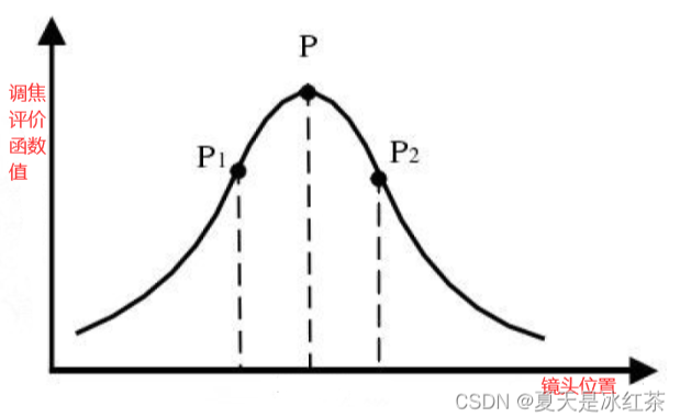
p点对应于正焦位置,P1 和P2 为正焦位置焦前和焦后采集到图像的清晰度评价结果。
正焦的图像比模糊的离焦图像边缘要更加的锐利清晰,相应的边缘像素灰度值变化大,因而会有更大的梯度值,从数学的角度来看图像,它是二维的离散矩阵,利用梯度函数可获取图像的灰度信息,来判别图像的清晰度,在离散信中梯度表现为差分形式。
传统的图像模糊检测主要存在以下缺点:
1.模糊界限难以确定,需要定一个阈值去区分(根据应用场景确定)。
2.众多的算法那个算法更适合,需要去验证。
针对传统算法也有一些机器学习和深度学习的方法去解决:
模糊度分类
1、运动模糊
运动模糊是在捕获图像时,快门在打开时间内成像系统和拍摄 对象的短暂相对运动,造成成像在某个方向上形成的模糊。
2、压缩模糊
压缩模糊是图像在进行有损压缩丢失部分信息。
3、高斯模糊
高斯模糊是人为引入的一种模糊,使用高斯低通滤波器对原始图像进行滤波得到的。
具体方法
传统算法
Brenner梯度法
计算相差两个单元的两个像素点的灰度差:

f(x,y) 表示图像f对应像素点(x,y)的灰度值,D(f)为图像清晰度计算结果。
python实现:
def brenner(img):
    '''
    :param img:narray 二维灰度图像
    :return: int 图像越清晰越大
    '''
    shapes = np.shape(img)
    output = 0
    for x in range(0, shapes[0]-2):
        for y in range(0, shapes[1]):
            output+=(int(img[x+2,y])-int(img[x,y]))**2
    return output
Tenegrad梯度法^3
传统的图像清晰度评价算法:
Tenengrad 梯度函数
Tenengrad 梯度函数采用Sobel算子分别提取水平和垂直方向的梯度值,基与Tenengrad 梯度函数的图像清晰度定义如下:

G(x,y) 的形式如下:
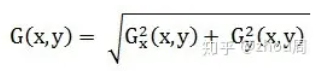
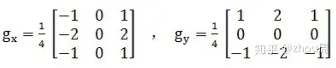
其中:T是给定的边缘检测阈值,Gx和Gy分别是像素点(x,y)处Sobel水平和垂直方向边缘检测算子的卷积,建议使用以下的Sobel算子模板来检测边缘:
laplace梯度法
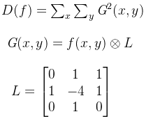
采用Laplace算子与图像各个像素点的灰度值进行卷积得到一个梯度矩阵记为G(x,y),取各像素点梯度的平方和作为评价函数,如下式所示:
def Laplacian(img):
    '''
    :param img:narray 二维灰度图像
    :return: int 图像越清晰越大
    '''
    return cv2.Laplacian(img,cv2.CV_64F).var()
方差法
聚焦清晰的图像比模糊图像有更大的灰度差异,可用方差函数作为评价:Fvariance=∑M∑N(f(x,y)−E2)
式中E为整幅图像的平均灰度值,该函数对噪声敏感。
能量梯度法
将 x 方向和 y 方向的相邻像素的灰度值之差的平方和作为每个像素点的梯度值,对所有像素梯度值累加作为清晰度评价函数值,表达式如下所示:

def EOG(img):
    '''
    :param img:narray 二维灰度图像
    :return: int 图像越清晰越大
    '''
    shapes = np.shape(img)
    output = 0
    for x in range(0, shapes[0]-1):
        for y in range(0, shapes[1]-1):
            output+=((int(img[x+1,y])-int(img[x,y]))**2+(int(img[x,y+1])-int(img[x,y]))**2)
    return output
roberts
Roberts函数与能量梯度函数相似,它是利用对角方向像素点灰度值之差。将4个相邻像素点的灰度值交叉相减的平方和作为每个像素点的梯度值,对所有像素梯度值累加作为清晰度评价函数值,表达式如下式所示:

def Roberts(img):
    '''
    :param img:narray 二维灰度图像
    :return: int 图像越清晰越大
    '''
    shapes = np.shape(img)
    output = 0
    for x in range(0, shapes[0]-1):
        for y in range(0, shapes[1]-1):
            output+=((int(img[x+1,y+1])-int(img[x,y]))**2+(int(img[x+1,y])-int(img[x,y+1]))**2)
    return output
SMD
当完全聚焦时,图像最清晰,图像中的高频分量也最多,故可将灰度变化作为聚焦评价的依据,灰度方差法的公式如下:

def SMD(img):
    '''
    :param img:narray 二维灰度图像
    :return: int 图像越清晰越大
    '''
    shape = np.shape(img)
    output = 0
    for x in range(1, shape[0]-1):
        for y in range(0, shape[1]):
            output+=math.fabs(int(img[x,y])-int(img[x,y-1]))
            output+=math.fabs(int(img[x,y]-int(img[x+1,y])))
    return output
SMD2 (灰度方差乘积)函数
SMD函数具有较好的计算性能,但其缺点也很明显,即在焦点附近灵敏度不高,即该函数在极值点附近过于平坦,从而导致聚焦精度难以提高。在《一种快速高灵敏度聚焦评价函数》中李郁峰等人在论文中提出了一种新的评价函数,称之为灰度方差乘积法,即对每一个像素领域两个灰度差相乘后再逐个像素累加,该函数定义如下:

def SMD2(img):
    '''
    :param img:narray 二维灰度图像
    :return: int 图像约清晰越大
    '''
    shape = np.shape(img)
    output = 0
    for x in range(0, shape[0]-1):
        for y in range(0, shape[1]-1):
            output+=math.fabs(int(img[x,y])-int(img[x+1,y]))*math.fabs(int(img[x,y]-int(img[x,y+1])))
    return output
Vollath函数

其中:μ为整幅图像的平均灰度值,M和N分别为图像宽和高。
#Vollath函数计算
def Vollath(img):
    '''
    :param img:narray 二维灰度图像
    :return: float 图像越清晰越大
    '''
    shape = np.shape(img)
    u = np.mean(img)
    out = -shape[0]*shape[1]*(u**2)
    for x in range(0, shape[0]-1):
        for y in range(0, shape[1]):
            out+=int(img[x,y])*int(img[x+1,y])
    return out
熵函数
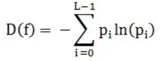
基于统计特征的熵函数是衡量图像信息丰富程度的一个重要指标,有信息论可知,一幅图像 f 的信息量是由该图像的信息熵 D(f) 来度量:
#entropy函数计算
def entropy(img):
    '''
    :param img:narray 二维灰度图像
    :return: float 图像越清晰越大
    '''
    out = 0
    count = np.shape(img)[0]*np.shape(img)[1]
    p = np.bincount(np.array(img).flatten())
    for i in range(0, len(p)):
        if p[i]!=0:
            out-=p[i]*math.log(p[i]/count)/count
    return out
深度学习
SVM 法1
- 使用拉普拉斯滤镜在输入图像中查找边缘
- 计算方差和已过滤图像像素值的最大值
- 高方差(和高最大值)表明边缘清晰可见,即图像清晰。低方差表明图像模糊。
- 基于Laplace的特征的图,我们注意到我们的两类(模糊和非模糊)是线性可分离的,然后利用SVM进行
#计算laplace算子
import numpy as np
from scipy.ndimage import variance
from skimage import io
from skimage.color import rgb2gray
from skimage.filters import laplace
from skimage.transform import resize

# Load image
path = f'test_data/0001.jpg'
img = io.imread(path)

# Resize image
img = resize(img, (400, 600))

# Grayscale image
img = rgb2gray(img)

# Edge detection
edge_laplace = laplace(img, ksize=3)

# Print output
print(f"Variance: {variance(edge_laplace)}")
print(f"Maximum : {np.amax(edge_laplace)}")
#利用SVM进行分类
import numpy as np

from sklearn import preprocessing, svm

# start with the results from the previous script
sharp_laplaces = [ (variance(edge_laplace_sharp_1), np.amax(edge_laplace_sharp_1)), ... ]
blurry_laplaces = [ (variance(edge_laplace_blurry_1), np.amax(edge_laplace_blurry_1)), ... ]

# set class labels (non-blurry / blurry) and prepare features
y = np.concatenate((np.ones((25, )), np.zeros((25, ))), axis=0)
laplaces = np.concatenate((np.array(sharp_laplaces), np.array(blurry_laplaces)), axis=0)

# scale features
laplaces = preprocessing.scale(laplaces)

# train the classifier (support vector machine)
clf = svm.SVC(kernel='linear', C=100000)
clf.fit(laplaces, y)

# print parameters
print(f'Weights: {clf.coef_[0]}')
print(f'Intercept: {clf.intercept_}')

# make sample predictions
clf.predict([[0.00040431, 0.1602369]])  # result: 0 (blurred)
clf.predict([[0.00530690, 0.7531759]])  # result: 1 (sharp)